Introduction

Welcome to your change in tandem and rates of change crash course review for AP® Precalculus! In this review, we’ll explore two essential sections: 1.1 Change in Tandem and 1.2 Rates of Change. These topics are fundamental for understanding how quantities vary together and how we can analyze these changes using functions. Whether you’re working on a graph or tackling a table of values, you’ll learn how to recognize relationships between inputs and outputs. After that, we’ll dive into comparing rates of change and building mathematical models.

Throughout this review, we’ll break down key concepts, walk through practical examples, and offer tips to help you master both change in tandem and rates of change. After you read through this review, click the button below to start 1.1 change in tandem practice set 1 on Albert.io.

1.1 Change in Tandem AP® Precalculus

1.1.A: Understanding How Input and Output Values Vary Together

Definition of a Function

A function is a rule that takes an input value (from the domain) and assigns it to a specific output value (in the range). Every input has exactly one output. The input is called the independent variable, and the output is known as the dependent variable because it depends on the input.

For example, consider a simple function like f(x) = 2x + 3 . Here, x is the independent variable (input), and f(x) is the dependent variable (output). If we input x = 2 , the function gives us an output of f(2) = 2(2) + 3 = 7 . So, for an input of 2, the corresponding output is 7.

How Input and Output Values Vary

The input and output values of a function change in tandem according to a specific function rule. You can express this rule in multiple ways:

• Graphically, by plotting points on a coordinate plane.
• Numerically, by using a table of values.
• Analytically, by writing an equation like f(x) = 2x + 3 .
• Verbally, by describing how the output changes as the input increases.

For instance, in the function f(x) = 2x + 3 , as x (the input) increases, the output, f(x) , also increases. We can express this change numerically:

x	f(x)
0	3
1	5
2	7
3	9

As you can see, as x increases by 1, the output increases by 2 each time.

Increasing and Decreasing Functions

A function is increasing over an interval if, as the input values increase, the output values also increase. For example, in the function f(x) = 2x + 3 , as x increases, f(x) increases as well. Formally, if a < b , then f(a) < f(b) .

In contrast, a function is decreasing over an interval if, as the input values increase, the output values decrease. Consider the function g(x) = -3x + 4 . As x increases, g(x) decreases because of the negative coefficient on x :

x	g(x)
0	4
1	1
2	-2
3	-5

In this case, as x increases, g(x) decreases.

1.1.B: Constructing Graphs for Contextual Scenarios

Visualizing Change in Tandem Relationships with Graphs

A graph represents how the input and output values of a function change together. Each point on the graph corresponds to an input-output pair (x, f(x)) . By looking at the graph, you can quickly see how input and output values change in tandem over an interval.

For example, the graph of f(x) = 2x + 3 is a straight line. You can plot some input-output pairs to create the graph:

x	f(x)
0	3
1	5
2	7

Plotting these points and drawing a line through them gives you a clear visual representation of how f(x) increases as x increases.

Using Verbal Descriptions to Construct Graphs

Sometimes, you may be given a verbal description of how two quantities change in tandem and need to construct a graph. For instance, imagine a car that accelerates from rest. Its speed starts at 0 and increases over time. You would expect the graph of speed (output) vs. time (input) to rise as time goes on. This describes an increasing function, where both input and output values rise together.

Concavity of Graphs

A graph is concave up on an interval if the rate of change is increasing. Visually, this looks like the graph curves upward like a bowl. This occurs when the function is accelerating, such as when an object speeds up faster and faster.

For example, a quadratic function like f(x) = x^2 is concave up because the rate of increase grows as x increases from left to right.

In contrast, a graph is concave down on an interval if the rate of change is decreasing. Visually, this looks like the graph curves downward like an upside-down bowl. For instance, a function like g(x) = -x^2 is concave down because, as we move left to right on the x-axis, the rates of change are decreasing from positive to zero to negative values.

Zeros of a Function

The zeros of a function occur when the output value equals zero. This happens where the graph intersects the x-axis. Zeros are significant because they represent moments where the dependent variable hits zero.

For instance, in the function h(x) = x - 2 , the zero occurs when h(x) = 0 . Solving for x , we find that x = 2 is the zero of the function, meaning the graph intersects the x-axis at (2, 0) .

1.2 Rates of Change AP® Precalculus

1.2.A: Comparing Rates of Change at Different Points

Average Rate of Change

The average rate of change measures how much the output of a function changes relative to the input over an interval. Mathematically, it’s the ratio of the change in output values to the change in input values.

The formula for the average rate of change of a function f(x) over the interval [a, b] is:

\text{Average rate of change} = \frac{f(b) - f(a)}{b - a}

For example, let’s take the function f(x) = x^2 and calculate the average rate of change between x = 1 and x = 3 . We plug these values into the formula:

\frac{f(3) - f(1)}{3 - 1} = \frac{9 - 1}{2} = 4

So, the average rate of change from x = 1 to x = 3 is 4.

Approximating the Rate of Change at a Point

The rate of change at a specific point tells us how fast the output is changing at that exact input. Although this exact rate requires calculus, we can approximate it by using average rates of change over smaller intervals near the point.

For instance, if we want to estimate the rate of change of f(x) = x^2 at x = 2 , we can calculate the average rate of change over smaller intervals around 2, like between x = 1.9 and x = 2.1 .

• f(1.9) = 1.9^2 = 3.61
• f(2.1) = 2.1^2 = 4.41

The approximate rate of change is:

\frac{f(2.1) - f(1.9)}{2.1 - 1.9} = \frac{4.41 - 3.61}{0.2} = 4

So, the rate of change at x = 2 is approximately 4.

Comparing Rates of Change at Two Points

To compare how fast a function is changing at two different points, we can look at their average rates of change over small intervals. If the average rate of change is larger at one point, it indicates that the output is changing faster at that input.

Let’s compare the rates of change of f(x) = x^2 at x = 1 and x = 3 :

At x = 1 , the average rate of change over x = 1 to x = 1.1 is:

\frac{f(1.1) - f(1)}{1.1 - 1} = \frac{1.21 - 1}{0.1} = 2.1

At x = 3 , the average rate of change over x = 3 to x = 3.1 is:

\frac{f(3.1) - f(3)}{3.1 - 3} = \frac{9.61 - 9}{0.1} = 6.1

This shows that the function is changing faster at x = 3 than at x = 1 .

1.2.B: Describing How Two Quantities Change in Tandem

Understanding Rates of Change

In section 1.2 rate of change, we learn more about how two quantities change in tandem. A positive rate of change indicates that as one quantity increases, the other also increases, or as one decreases, the other decreases as well.

For example, in the function f(x) = 2x , as x increases, f(x) increases too. This positive relationship means the function is increasing.

Positive and Negative Rates of Change

A positive rate of change means both quantities move in the same direction. If one increases, so does the other.

For instance, in the function f(x) = 3x , as x increases, f(x) increases as well. A real-world example might be the distance traveled by a car moving at constant speed: the more time passes, the greater the distance traveled.

A negative rate of change means the quantities move in opposite directions. If one increases, the other decreases.

For example, in the function g(x) = -2x , as x increases, g(x) decreases. This could represent a scenario like the temperature of a cooling object: as time passes, the temperature decreases.

Change in Tandem and Rates of Change: Sample AP® Questions

1.1 Change in Tandem Practice Set 1

Let’s take a look at some released change in tandem AP® Precalculus problems:

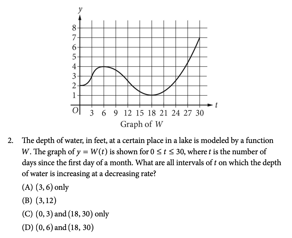
We are presented with the graph of W that models the depth of the water, in feet, in a lake. We need to identify which intervals of t show where the depth of the water is increasing at a decreasing rate. This means we need to identify where the function has a positive slope and which of those intervals occurs where the graph is concave down. Let’s look at all the intervals on the graph:

(0,3): Increasing & Concave Up

(3,6) : Increasing & Concave Down

(6,12) : Decreasing & Concave Down

(12,18) : Decreasing & Concave Up

(18,30) : Increasing & Concave Up

The only interval where the graph has a positive slope on an interval that is also concave down is (3,6) , so our answer is A. This is the interval where the depth of water is increasing at a decreasing rate.

1.1 Change in Tandem Practice Set 2

Our next change in tandem AP® Precalculus sample question comes from the calculator section of the released AP® Precalculus practice exam.

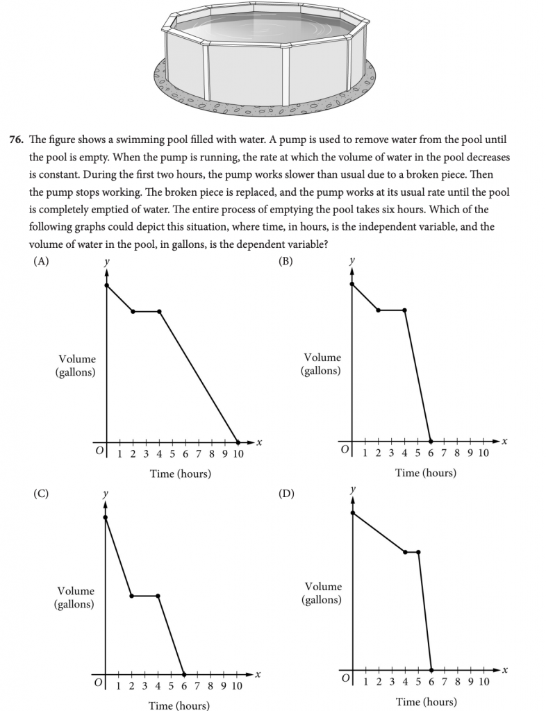
In this problem, we are given the verbal description of a function and how its rates change in tandem. We are then asked to identify the graph that could depict this situation. Let’s break it down:

“The rate at which the volume of water in the pool decreases is constant.”

This tells us that the graph is linear because linear graphs have a constant rate of change.

“During the first two hours, the pump works slower than usual due to a broken piece.”

From this information, we can assume that the slope from 0 to 2 will be slightly less negative than other intervals given because the volume is decreasing at a slower rate due to the broken piece.

“Then the pump stops working.”

Over this interval, we should see a line segment with a 0 slope, or constant volume, because the rate of change in volume will be 0 when the pump isn’t working.

“The broken piece is replaced, and the pump works at its usual rate until the pool is completely emptied of water.”

Now, we should see a slightly more negative slope because the rate at which volume is decreasing is faster than the first two hours because the pump is back to working order.

“The entire process of emptying the pool takes six hours.”

This final sentence is necessary to know that at six hours, the volume will be 0. This indicates that the graph should intersect the x-axis after six hours.

Putting this all together leaves us with B as the only correct option.

Conclusion

In this crash course for AP® Precalculus, we explored two important topics: 1.1 Change in Tandem and 1.2 Rates of Change. We began by looking at how input and output values vary together in functions. By analyzing functions through different representations—graphs, tables, equations, and verbal descriptions—you can better understand how input values affect outputs. We also discussed how functions can be increasing or decreasing and how to visualize these changes with graphs.

In Section 1.2, we took a closer look at rates of change, learning how to calculate the average rate of change and approximate the rate of change at specific points. You saw how positive rates of change indicate that two quantities move together in the same direction, while negative rates of change show them moving in opposite directions.

These concepts form the foundation for much of precalculus, helping you understand the dynamic relationships between quantities. As you move forward, remember to practice constructing graphs, comparing rates of change, and interpreting these variations in both real-world and mathematical contexts. And don’t forget to review the 1.1 Change in Tandem practice set 1 on Albert.io to reinforce these skills!

Need help preparing for your AP® Precalculus exam?

Albert has hundreds of AP® Precalculus practice questions, free response, and an ap precalculus practice test to try out.