
Graphing linear equations is an important Algebra skill. Just as painting a picture can help an artist express their emotions, creating a graph can help a mathematician explain and visualize a relationship.
In this article, we will review graphing a linear equation in two variables. We will review how to graph linear equations using two points, using intercepts, and using a slope and a y-intercept. Additionally, we will use transformations to graph linear equations. Graphing horizontal and vertical lines and the best online calculator tools for graphing are also topics we discuss. This post is full of graphing linear equation examples!
Let’s jump right in.
What We Review
Why do we graph linear equations?
Graphing linear equations creates a visual to explain the relationship between two variables. Using a graph we can easily see what happens to one variable as the other increases. As we move to the right on a graph, the value of the x variable increases. If the line moves up, the y variable also increases, but if the line moves down, the y variable decreases. If the line stays the same, this means the y variable does not change.
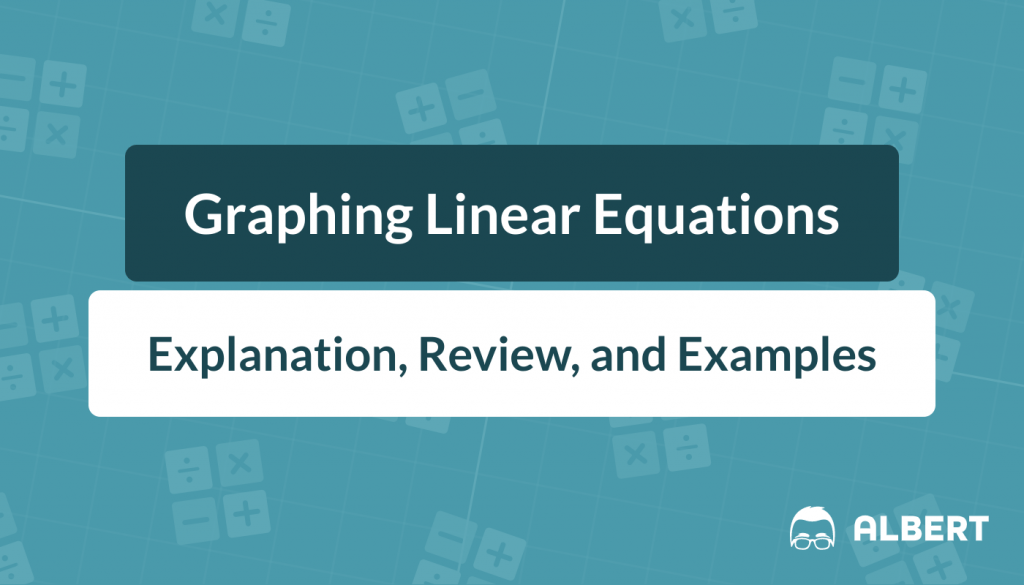
For example, let us suppose we are graphing the linear equations y=3x-1 and y=\frac{1}{2}x-1.
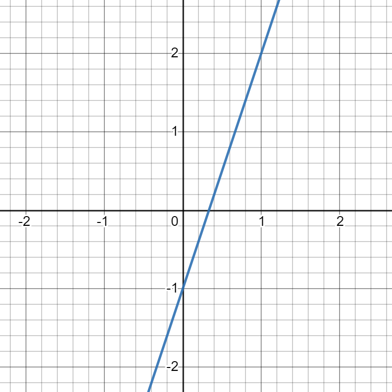
The images above more easily visualize the relationship between the variables for each graph. We see two positive slopes and the same y-intercept, -1. We can make comparisons between the graphs, noting that the graph of the linear equation y=3x-1 is steeper than y=\frac{1}{2}x=1.
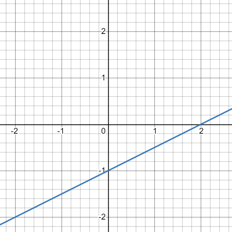
If we plot them together, we can also easily identify points of intersection (which is often called “the solution” of both lines).
In this case, the lines intersect at the point (0,-1) which is also their y-intercept.
To sum up, graphing can help mathematicians display relationships between two variables, compare characteristics between two graphs, and determine solution sets for linear equations.
Return to the Table of Contents
What form is best for graphing linear equations?
Using slope-intercept form can make graphing simple. In slope-intercept form, we easily identify the y-intercept and the slope of the graph. Using this form gives us a step-by-step process we can always use to create our graph.
As a reminder, here are the three common forms of linear equations:
| Slope-Intercept Form | y=mx+b | Review slope-intercept form |
| Point-Slope Form | y-y_1=m(x-x_1) | Review point-slope form |
| Standard Form | ax+by=c | Review standard form |
The m and b of slope-intercept form are the slope and y-intercept, respectively.
Point-slope form also uses m for the slope but may use any point on the line. Using slope-intercept form gives us the advantage of always starting with the y-intercept.
Standard form does not give us any information for our graph. We could eventually graph a line given in standard form but we would likely first need to convert to slope-intercept form.
Return to the Table of Contents
Use slope and y-intercept to graph linear equation (example)
There is a step-by-step process on how to graph linear equations in slope-intercept form, y=mx+b.
For example, we’ll graph the equation y=4x-2.
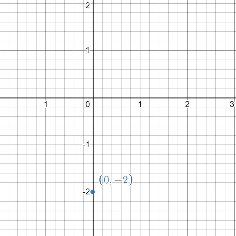
Step 1: Identify and graph the y-intercept.
We see that in our equation, y=4x-2, the number -2 is in the place of b. We will begin our graph by plotting the point (0,-2). Remember, the y-intercept is where the graph crosses the y-axis, so the x-coordinate is always 0.
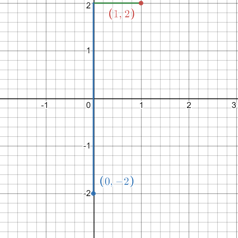
Step 2: Using the slope, identify the rise and the run
Slope can be expressed as \frac{rise}{run}. In our equation, y=4x-2, the number 4 is in the place of m. Therefore, the slope is 4 which can be expressed as \frac{4}{1}. This means the rise is 4 and the run is 1. In other words, the graph will rise 4 units up for every 1 unit it runs to the right.
Step 3: Use the rise and run to plot the next point.
We will count up 4 units and right 1 unit to plot the next point on our graph. This makes our next point at (1,2).
Return to the Table of Contents
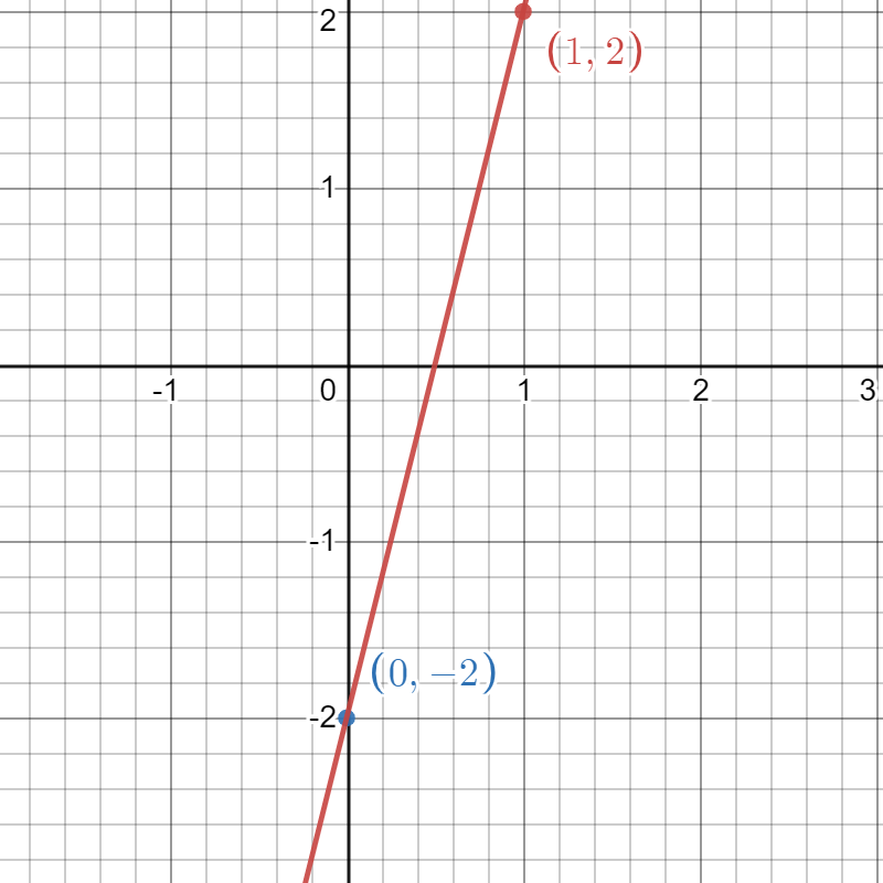
Step 4: Connect the two points.
Now, we make a line through the y-intercept of (0,-2) and the new point we have plotted, (1,2). This is the graph of the linear equation y=4x-2.
Return to the Table of Contents
Use two points to graph linear equation (example)
If we are given two points of a linear equation, we may simply graph the points and then connect the points.
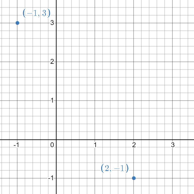
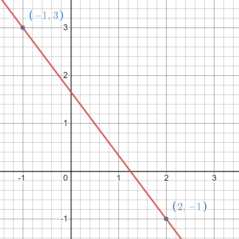
Let us graph the line which goes through the points (-1,3) and (2,-1).
First, for our example, we will plot the points.
Now, we will connect them with a line. This is the graph of the linear equation that goes through the two points (-1,3) and (2,-1).
Return to the Table of Contents
Use intercepts to graph linear equation (example)
We can use intercepts to graph linear equations in the same way we would use two points. Remember, the x and y-intercepts are also points on the graph.
Let us suppose we need to graph a linear equation with a y-intercept of 3 and an xintercept of 2. This tells us two points on the graph. We know the point (0,3) on the graph because the y-intercept is 3. We also know the point (2,0) is on the graph because the xintercept is 2.
Let us plot the two points we know.
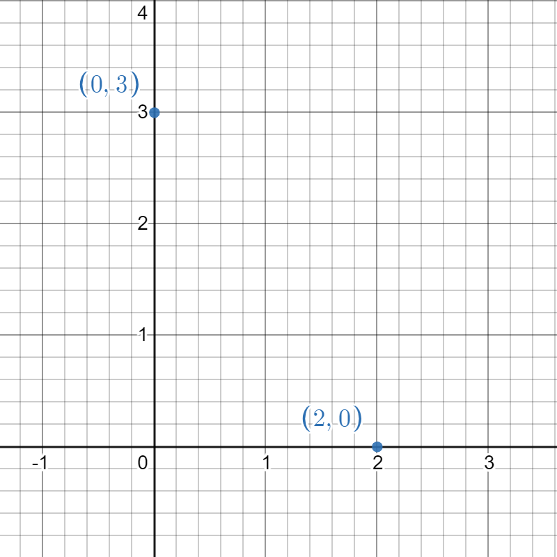
As before, we will connect the two points to create the graph of the linear equation.

This is how to create the graph of a linear equation using the intercepts.
Return to the Table of Contents
Use transformations to graph linear equation (example)
When graphing linear equations, we may need to use transformation to obtain a new graph. Let us begin with the graph we created of y=4x-2. Remember, this graph has a slope of 4 and a y-intercept of -2.

Let’s now consider the equation y=4x+1. We can see this equation has the same slope. Instead of starting the graphing process over, we can consider how this graph has changed.
We see that the y-intercept changed from -2 to 1. The difference between -2 and 1 is 3. We can determine this with subtraction: 1-(-2)=3. We know the graph was transformed up 3.
To make this more clear, let us examine the equations. The original graph is of y=4x-2. If we add 3 to this graph, we obtain y=4x-2+3 which gives us the new equation y=4x+1. We can use this information to make the new graph. All we need to do is more our points up 3 units.
Instead of graphing (0,-2), we will graph (0,-2+3) which is (0,1). Remember, moving a graph up only changes the y-coordinate.
Likewise, instead of graphing (1,2), we will graph (1,2+3 which is (1,5).
Let us plot the points (0,1) and (1,5) and connect them.
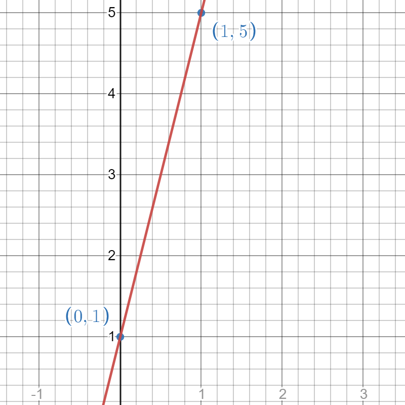
We’ve now used transformations to create the graph of the linear equation y=4x+1.
Return to the Table of Contents
How to graph horizontal and vertical lines
Graph a horizontal line
Graphing horizontal and vertical lines is a little bit different because these equations do not look like we expect them to.
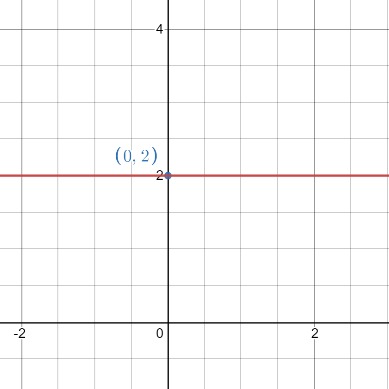
Let us begin with a horizontal line. We will create the graph of the horizontal line y=2. Horizontal lines are always in the form y=a where a represents a real number. It may be hard to see it, but this equation is actually in point-slope form. It just has a slope of zero. We can think of it like this: y=0x+2.
All horizontal lines have a slope of zero. First, we will plot the point (0,2). When the line starts with y=, we will begin by plotting a point on the y-axis. We know (0,2) is on the graph because the y-coordinate is 2.
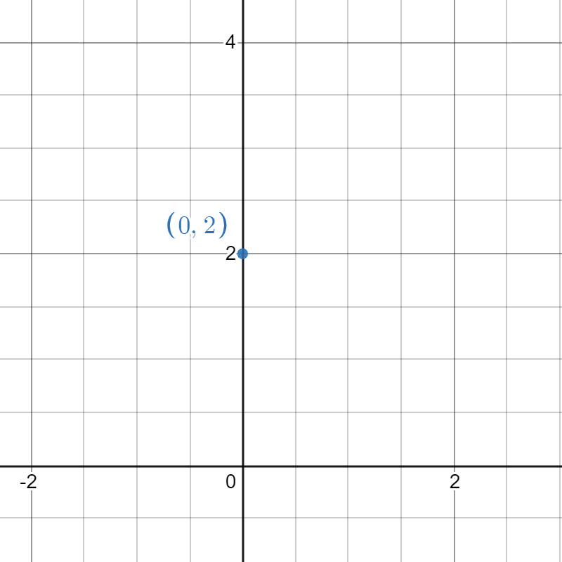
Now, we create the horizontal line through the point (0,2). At all values on this line, the y-coordinate is 2. This is the graph of the horizontal line y=2.
Graph a vertical line
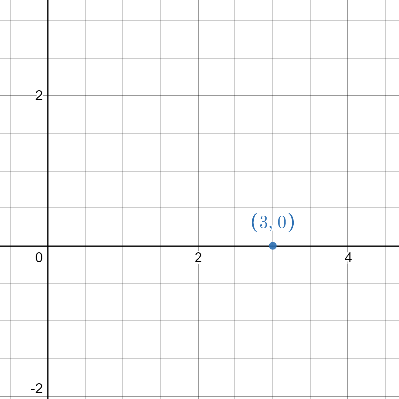
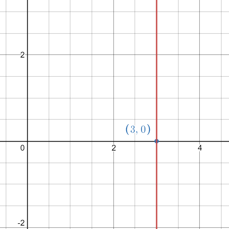
We can now graph a vertical line. We will create the graph of the vertical line x=3. Vertical lines are always in the form x=a where a represents a real number. Vertical lines are never in point-slope form, slope-intercept form, or standard form. This is because a vertical line has a slope that is undefined, so it cannot fit any of these forms.
First, we will plot the point (3,0). When the line starts with x=, we will begin by plotting a point on the x-axis. We know (3,0) is on the graph because the x-coordinate is 3.
Now, we create the vertical line through the point (3,0). At all values on this line, the x-coordinate is 3. This is the graph of the vertical line x=3.
This is the process used for graphing horizontal and vertical lines.
Return to the Table of Contents
Top 3 online calculators for graphing linear equations
To get more online practice graphing equations, try using these resources:
Desmos.com
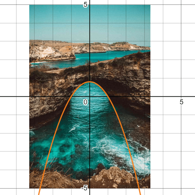
At Desmos, you have many options to customize your graph! This tool is very user-friendly. You can manipulate equations to understand how the different parts influence the graph. You can graph multiple lines at a time. Desmos even allows photographs to be included in a graph, like this:
Geogebra.org
At Geogebra, you are also able to graph many different types of equations. Exploring Geogebra, you will also find excellent tools for creating geometric figures.
Meta-calculator.com
Using Meta-calculator feels more like using a traditional calculator. This may help you feel more comfortable using a handheld graphing calculator in class.
Return to the Table of Contents
Summary: Graphing with Linear Equations
In this post, we’ve learned a lot about graphing linear equations.
- We can graph linear equations to show relationships, compare graphs, and find solutions.
- Point-slope form is the best form to use to graph linear equations .
- We can create a graph using slope and y-intercept, two points, or two intercepts.
- Lots of great graphing calculator resources are available online, like Desmos, Geogebra, and Meta-calculator.
Click here to explore more helpful Albert Algebra 1 review guides.


