Statistics has a habit of taking words that we know and love, and turning them into something else completely. Take the range, for example. While this term may make you think of the old tune “Home on the Range,” the definition of range in math involves way fewer deer and antelope. Luckily for you, this AP® Statistics review is here to save you from confusion. Read on to learn what a range is and why it’s important, how to calculate a range, and how to tackle range-related questions on the AP® Stats exam. By the end of this article, you’ll be at home on the range!
What is a Range?
Below is a picture of what you might imagine when you hear the word “range” – a wide, open stretch of land. In a way, a connection can be made to the meaning of range in math: it’s the stretch of your data set, the distance from one side of your distribution to the other. It’s a descriptive statistic, which is exactly what it sounds like – it helps to describe the shape of a distribution. In this case, range tells us how wide or spread out a distribution is. Just like they preferred it in the Old West, the range is a simple idea, and calculating the range is just as easy. Which brings us right along to the next point…

How to Calculate the Range
In its most basic form, the range is simply the numeric distance between the smallest and largest values in your distribution. At this point, calculating it is probably obvious: you just subtract the smallest number from the largest! Just for fun, let’s try out an example. Say we have a class of 5 students, and their AP® Stats test has just been returned. Their scores looked like this:
| Student 1 | Student 2 | Student 3 | Student 4 | Student 5 |
| 90% | 75% | 82% | 98% | 40% |
The first step is to locate our smallest and largest values – easy peasy! Since that’s so simple, we might as well arrange the data into numerical order, as that may help us later on if we want to calculate other things, like the median (see our post on the median for a review of that concept).
| Student 5 | Student 2 | Student 3 | Student 1 | Student 4 |
| 40% | 75% | 82% | 90% | 98% |
Then, we take our largest value and subtract our smallest value:
98 – 40 = 58
So our range is 58%. It’s that simple! In fact, the range can also be expressed in another, even easier way: 40% to 98%.
While the first method is more common, this second way of expressing the range is useful when the problem also requires you to know the exact values of the endpoints, rather than just the distance between them. Which version you use will depend on upon the problem.
Why do We Calculate the Range?
As you can see, the range gives us an idea of how spread out our distribution is. The various measures of spread, including the range, are referred to in AP® Stats as measures of “variance.” The term variance refers to how much your scores vary – are they all pretty similar and packed together, or do they differ by a large amount? Let’s look at some examples to better understand the concept of variance.
First, imagine your class takes a test that is incredibly easy. Everyone in the class is likely to do very well. The scores might look like this:
| Student 1 | Student 2 | Student 3 | Student 4 | Student 5 |
| 98% | 100% | 99% | 100% | 97% |
The range, in this case, is 100 – 97 = 3.
Next, suppose the same students take a different test that is extremely difficult, and everyone does poorly. The scores might look like this:
| Student 1 | Student 2 | Student 3 | Student 4 | Student 5 |
| 65% | 67% | 66% | 67% | 64% |
When we calculate our range: 67 – 64 = 3.
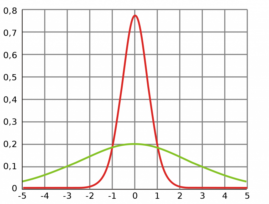
The range is exactly the same in both cases, even though the scores are very different! That’s because the shape of the distribution hasn’t changed, it has simply been shifted over to the left. In other words, the range doesn’t reflect the absolute value of your scores, just the relative differences among them. In both of these examples, the scores are packed in close together. Another way of saying this is that the variance is low. Conversely, in the first example above, we had some scores that were low and some that were high. In that case, the variance is much greater. The image below illustrates this: the skinny distribution has low variance (and therefore a small range), while the fat distribution has high variance (and a large range).
Problems with Using the Standard Range
Every statistic has its pros and cons – each is useful in certain situations, but not in others. For example, in a previous post we discussed how the mean is pulled by the extremes, and so we may want to use the median in cases where the distribution is asymmetrical or has outliers. The standard range faces a similar issue. Consider the following: Imagine the same situation as the last example, in which we have a very difficult test and 5 students all do pretty poorly on it. However, this time, suppose we add a sixth student who did extremely well (smells like a cheater to me…). The data could look like this:
| Student 1 | Student 2 | Student 3 | Student 4 | Student 5 | Student 6 |
| 65% | 67% | 66% | 67% | 64% | 100% |
Then we calculate the range: 100 – 64 = 36.
With the addition of this single outlier, the range has jumped from 3% to 36%! This new number is a very poor indication of the variance in our scores. If we were to look at that number alone, we would expect the scores to be pretty spread out. However, 5 out of 6 scores are still packed in close together, and only one is far apart. This example illustrates how the range is influenced by outliers.
Enter the Interquartile Range (IQR)
That’s where the interquartile range comes into play. The IQR is when you take a range but ignore the top 25% and bottom 25% of the data so that any outliers will be cut out. As a result, it identifies the middle 50% of your data set and may provide a better description of the variance in your data.
When you hear “quartiles,” think “quarters” or dividing scores into four even chunks. You accomplish this process using the same technique we used to find the median. Here are the steps for how to calculate the interquartile range:
• Arrange your data in numerical order.
• Find the median (which is also { Q }_{ 2 }) – your data is now split in half
• Find a “median” for each of the halves ({ Q }_{ 1 } and { Q }_{ 3 })
• The IQR is the range between { Q }_{ 1 } and { Q }_{ 3 } – simply subtract the smaller from the larger as we did before.
The dividing lines of your quartiles are called { Q }_{ 1 }, { Q }_{ 2 }, and { Q }_{ 3 }. It may seem strange at first that there are only 3 of these, but imagine taking a small rope and cutting it into 4 pieces. How many cuts would you have to make? Only 3, since the last cut will result in 2 pieces.
Let’s try this with a concrete example. This time, we will use 11 students to make the math simpler. Below we have the test scores for 11 students.
| Student 1 | Student 2 | Student 3 | Student 4 | Student 5 | Student 6 | Student 7 | Student 8 | Student 9 | Student 10 | Student 11 |
| 70% | 98% | 67% | 82% | 100% | 85% | 79% | 89% | 87% | 84% | 86% |
First, we rearrange the data to be in numerical order:
| Student 3 | Student 1 | Student 7 | Student 4 | Student 10 | Student 6 | Student 11 | Student 9 | Student 8 | Student 2 | Student 5 |
| 67 | 70 | 79 | 82 | 84 | 85 | 86 | 87 | 89 | 98 | 100 |
Then, we find the median as well as { Q }_{ 1 } and { Q }_{ 3 }.
| Student 3 | Student 1 |
Student 7 |
Student 4 | Student 10 |
Student 6 |
Student 11 | Student 9 |
Student 8 |
Student 2 | Student 5 |
| 67 | 70 |
79 |
82 | 84 |
85 |
86 | 87 |
89 |
98 | 100 |
As you can see, { Q }_{ 2 } is the value directly in the middle, and { Q }_{ 1 } and { Q }_{ 3 } are the values in the middle of their respective halves. Now, the IQR is simply the range from { Q }_{ 1 } to { Q }_{ 3 }.
89 – 79 = 10
In this example, most of the scores are between 79-89%, but a couple of students got scores much lower, and a couple got scores much higher. Those scores are outliers and would expand our range to be much bigger. As a result, the IQR provides a more accurate picture of our data in this case.
Now, the example above was designed to have easy to find quartiles, but what if our data don’t divide easily? For example, imagine we have 5 data points again.
| Student 5 | Student 2 |
Student 3 |
Student 1 | Student 4 |
| 40 | 75 |
82 |
90 | 98 |
In this case, our median is simple to find, but our { Q }_{ 1 } and { Q }_{ 3 } will fall between two values. To get around this, we use the same logic as when this happens with the median – you simply find the number that is directly between those values by taking the mean.
{ Q }_{ 1 } is between the first two values, so:\dfrac{40+75}{2}=57.5.
{ Q }_{ 3 } falls between the last two values, so:\dfrac{90+98}{2}=94.
Then, our IQR is
{ Q }_{ 3 } – { Q }_{ 1 }: 94 – 57.5 = 36.5.
Using Ranges on the AP® Statistics Exam
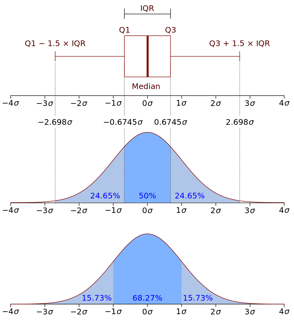
The most common reason to calculate range on the AP® Stats exam will be for a boxplot, also known as a “box and stem” graph (see the image above for an example). Boxplots give a detailed description of your data because they include several different values: the standard range, the IQR, and the median. The “box” represents the IQR, the line in the center of the box represents the median, and the “stems” represent the full range. This representation allows the viewer to get an accurate picture of the variance as well as the outliers, and provides a measure of the central value.
From this AP® Stats review, you now know what a range is, how to calculate ranges and IQR’s, why they’re important, and how to use them on the AP® exam! At this point, you should have a handle on the main methods for describing distributions, including measures of central tendency and variance. With these foundational concepts nailed down, you’ve laid the groundwork for the rest of AP® Statistics!
Looking for more AP® Statistics practice?
Check out our other articles on AP® Statistics.
You can also find thousands of practice questions on Albert.io. Albert.io lets you customize your learning experience to target practice where you need the most help. We’ll give you challenging practice questions to help you achieve mastery of the AP® Statistics.
Start practicing here.
Are you a teacher or administrator interested in boosting AP® Statistics student outcomes?
Learn more about our school licenses here.


