What is Stokes’ Theorem about?
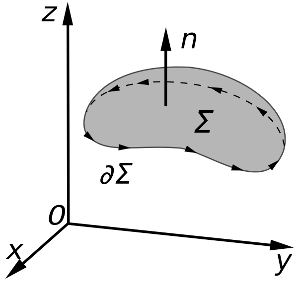
Stokes’ Theorem is about tiny spirals of circulation that occurs within a vector field (F). The vector field is on a surface (S) that is piecewise-smooth. Additionally, the surface is bounded by a curve (C). The curve must be simple, closed, and also piecewise-smooth. Stokes’ theorem equates a surface integral of the curl of a vector field to a 3-dimensional line integral of a vector field around the boundary of the surface. It basically says that the surface integral of curl F over a surface is the circulation of F around the boundary of the surface.
If this sounds somewhat familiar, it might be because it is. Stokes’ Theorem is a generalization of Green’s Theorem to three dimensions. Green’s Theorem says that given a continuously differentiable two-dimensional vector field F, the circulation of F over some region bounded by a simple closed curve is equal to the total circulation of F around the curve. That is, it equates a 2-dimensional line integral to a double integral of curl F.
So from Green’s Theorem to Stokes’ Theorem we added a dimension, focus on a surface and its boundary, and speak of a surface integral instead of a double integral.
Formal Definition of Stokes’ Theorem
Given:
• an oriented, piece-wise smooth surface (S)
• a simple, closed, piece-wise-smooth curve (C) that bounds S
• a continuously-differentiable vector field (F) in 3-D space that contains S
Stokes’ Theorem states: o\int_{ C }^F\cdot ds=i\int _{ S }^{ curlF \cdot } dS
A Note on Orientation
In order for Stokes’ Theorem to work (and for you to avoid getting the sign wrong as you work through examples) the boundary of the surface (C) has to be positively oriented. There are two ways we can check the orientation (neither of which seem to have to do with math though they actually do).
• Use your right hand: A boundary surface is positively oriented if when your thumb is pointed in the direction of the surface normal, the other fingers (those that are curled up) are in the direction of the surface. Think about the curled up fingers being where the swirls within the surface are and the outside of your hand is where the boundary lies.
• Go for a walk near a lake: You might have to picture this one in your head depending on where you live. The idea here is that the normal vector points straight up to the sky. You are walking along the edge of the lake (think of this as the boundary of the surface and the lake can be the surface). The boundary of the surface is positively oriented if the lake is always to your left as you walk along the edge. And yes, you can only walk along the ground (not under or above it) so this model might not be the most accurate, but it should help in terms of visualizing what we mean by the boundary must be positively oriented.
What’s so Great about Stokes’ Theorem?
Stokes’ Theorem is true regardless of the surface we choose provided that the surface is oriented a certain way, it is piece-wise, and it is smooth. This is extremely powerful as it means that the relationship is true irrespective of the surface. What does that mean for you? It means that when you have to evaluate one of these integrals you can choose a surface that is convenient (ie. makes the mathematical computations easier to do).
The other great thing is that you now have options. You can find a 3-D line integral or, if it is easier, the surface integral. Knowing this equality exists means that if you are asked for one side of the equation, you can choose to use the other if it is more convenient (that is, easier for you to do).
How to Use Stokes’ Theorem – Two Examples
Example 1: Let C be the circular sector in the diagram below.
The coordinates of A, B, and C are (0, 0, 0),\left( 0,\dfrac { 3 }{ 2 } ,\dfrac { 3\sqrt { 3 } }{ 2 } \right) and \left( 0,\dfrac { 3\sqrt { 3 } }{ 2 } ,\dfrac { 3 }{ 2 } \right) respectively. Note that the sector makes an angle of \dfrac{\pi}{6} radians with both the y and z axes.
For F=(y,z,x) compute o\int _{ C }^{ }{ F\cdot ds } using Stokes’ Theorem.
We are given the line integral and told to use Stokes’ Theorem. That means that instead of finding the line integral directly, we are being asked to find the surface integral that corresponds to the line integral given. That is, we need to find i\int_{ S }^{ }{ curlF } \cdot dS.
Before we can compute the surface integral, here’s what we need to find:
The surface S with a positively oriented boundary C
Curl F
An equation for S
The normal vector
Let’s find each.
The surface S
We need a surface with boundary C such that C is a positively oriented boundary. The circular sector itself is a good choice. As we travel from A to B to C, we keep the surface to our left if the normal vector points to the negative side of the x-axis.
Finding Curl F
We need to find curl F and do so as follows.
\begin{vmatrix} i& j & k \dfrac{ \partial }{ \partial x } &\dfrac { \partial }{ \partial y } &\dfrac { \partial }{ \partial z } \ y & z & x \end {vmatrix}
=i\left( \dfrac { \partial }{ \partial y } x-\dfrac { \partial }{ \partial z } z \right) -j\left( \dfrac { \partial }{ \partial x } x-\dfrac { \partial }{ \partial z } y \right) +k\left( \dfrac { \partial }{ \partial x } z-\dfrac { \partial }{ \partial z } z \right)
=(-1,-1,-1)
If the above felt like to big a jump, you might want to go back to review how to find the determinant of a three by three matrix and/or how to take a partial derivative.
Finding an equation for S
We need an equation for the surface we selected. Namely, we need an equation for the circular sector in the diagram. We use a parametric equation as follows.
S(r,\theta )=(0,rcos\theta ,rsin\theta ) where r runs from 0 to the distance from the origin to point B and \theta runs from \dfrac { \pi }{ 6 } (the angle between the y-axis and the sector) and \dfrac { \pi }{ 3 } leaving an angle between the sector and the z-axis of \dfrac { pi }{ 6 } as well.Putting this together we obtain S(r,\theta )=(0,rcos\theta ,rsin\theta ) for 0\le r\le 3 and \dfrac { \pi }{ 6 }\le \theta \le \dfrac { \pi }{ 2 }.
Finding the normal vector
We find the normal vector as follows.
\dfrac { \partial D }{ \partial r } =(0,cos\theta ,sin\theta )
\dfrac { \partial D }{ \partial \theta } =(0,-rsin\theta ,rcos\theta )
\dfrac { \partial D }{ \partial r } \times \dfrac { \partial D }{ \partial \theta } =i(r{ cos }^{ 2 }\theta +i{ sin }^{ 2 }\theta )=ri
There is one problem here. The vector we found points in the direction of the positive x-axis and prior we noted that the normal vector must point towards the negative x-axis. We can correct this, by using the normal vector -ri
Now that we have everything we need, let’s compute the surface integral.
o\int _{ C }^{ }{ F } =i\int _{ S }^{ }{ curlF\cdot } dS
=\int _{ 0 }^{ 3 }{ \int _{ \pi /6 }^{ \pi /3 }{ (-1,-1,-1)\cdot (-r,0,0)d\theta dr } }
=\int _{ 0 }^{ 3 }{ \int _{ \pi /6 }^{ \pi /3 }{ rd\theta dr } }
=\int _{ 0 }^{ 3 }{ { \left[ r\theta \right] }_{ \pi /6 }^{ \pi /3 } } dr
=\int _{ 0 }^{ 3 }{ \left[ r\left( \dfrac { \pi }{ 3 } \right) -r\left( \dfrac { \pi }{ 6 } \right) \right] } dr
=\int _{ 0 }^{ 3 }{ \dfrac { r\pi }{ 6 } dr }
={ \left[ \left( \dfrac { \pi }{ 6 } \right) \left( \dfrac { { r }^{ 2 } }{ 2 } \right) \right] }_{ 0 }^{ 3 }
=\left( \dfrac { \pi }{ 6 } \right) \left( \dfrac { { 3 }^{ 2 } }{ 2 } \right) -0
=\dfrac { 9\pi }{ 12 }
=\dfrac { 3\pi }{ 4 }
Example 2: Let C be the circular sector in the diagram below. The coordinates of A, B, and C are (0, 0, 0),\left( 0,\dfrac { 3 }{ 2 } ,\dfrac { 3\sqrt { 3 } }{ 2 } \right) and \left( 0,\dfrac { 3\sqrt { 3 } }{ 2 } ,\dfrac { 3 }{ 2 } \right) respectively. Note that the sector makes an angle of \dfrac{\pi}{6} radians with both the y and z axes.
For F=(y,z,x) compute i\int _{ S }^{ }{ curlF } \cdot dS
Everything here is the same as in example 1. The difference is that you are being given the surface integral and since you are asked to use Stokes’ Theorem instead of finding it directly, we use the line integral.
To find the line integral we need an equation for the boundary C. It helps to break that up into three pieces. C1 takes us from A to B. C2 takes us from B to C. C3 takes us from C to A.
Let’s start with the line integral over C1.
The angle between the y-axis and C1 is \dfrac{ \pi }{ 3 } making the slope of the segment tan\dfrac { \pi }{ 3 } =\sqrt { 3 } and giving rise to the following parametrization.
c(t)=(0,t,t\sqrt { 3 } ),0\le t\le \dfrac { 3 }{ 2 }
As a result, { c }^{ ' }(t)=(o,1,\sqrt {3 } ) and so F(c(t))\cdot c'(t)=F(0,t,t\sqrt { 3 } )\cdot (0,1,\sqrt { 3 } )=t\sqrt { 3 }.
That means that
\int _{ { c }_{ 1 } }^{ }{ F\cdot ds=\int _{ 0 }^{ 3/2 }{ t\sqrt { 3 } } } dt
={ \left[ \dfrac { { t }^{ 2 }\sqrt { 3 } }{ 2 } \right] }_{ 0 }^{ 3/2 }
=\left( \dfrac { \sqrt { 3 } }{ 2 } \right) { \left( \dfrac { 3 }{ 2 } \right) }^{ 2 }-0
=\dfrac { 9\sqrt { 3 } }{ 8 }
Similarly, the line integral over C3 can be found as follows:
The angle between the y-axis and C3 is \dfrac{ \pi }{ 6 } making the slope of the segment tan\frac { \pi }{ 3 } =\dfrac { \sqrt { 3 } }{ 3 } and giving rise to the following parametrization.
c(t)=(0,t,\dfrac { t\sqrt { 3 } }{ 3 } ),0\le t\le \dfrac { 3\sqrt { 3 } }{ 2 }.
As a result, { c }^{ ' }(t)=(o,1,\dfrac { \sqrt { 3 } }{ 3 } ) and so F(c(t))\cdot c'(t)=F(0,t,\dfrac { t\sqrt { 3 } }{ 3 } )\cdot (0,1,\dfrac { \sqrt { 3 } }{ 3 } )=\dfrac { t\sqrt { 3 } }{ 3 }.
That means that
\int _{ { c }_{ 2 } }^{ }{ F\cdot ds=\int _{ (3\sqrt { 3 } )/2 }^{ 0 }{ \dfrac { t\sqrt { 3 } }{ 3 } } } dt
={ \left[ \left( \dfrac { \sqrt { 3 } }{ 3 } \right) \dfrac { { t }^{ 2 } }{ 2 } \right] }_{ (3\sqrt { 3 } )/2 }^{ 0 }
=0-\left( \dfrac { \sqrt { 3 } }{ 3 } \right) { \left( \dfrac { 1 }{ 2 } \right) \left( \dfrac { 3\sqrt { 3 } }{ 2 } \right) }^{ 2 }-0
=\dfrac { -9\sqrt { 3 } }{ 8 }
Lastly we consider the line integral over C2.
Here c(t)=(0,rsint,rcost),\dfrac { \pi }{ 6 } \le t\le \dfrac { \pi }{ 3 } That means that c'(t)=(0,rcost,-rsint)
Further:
\int _{ C_{ 2 } }^{ }{ F\cdot ds=\int _{ \dfrac { \pi }{ 6 } }^{ \dfrac { \pi }{ 3 } }{ F(c(t))\cdot c'(t)dt } }
=\int _{ \dfrac { \pi }{ 6 } }^{ \dfrac { \pi }{ 3 } }{ F(0,rsint,rcost)\cdot (0,rcost,-rsint)dt }
=\int _{ \dfrac { \pi }{ 3 } }^{ \dfrac { \pi }{ 3 } }{ (rsint,rcost,0)\cdot (0,rcost,-rsint)dt }
=\int _{ \frac { \pi }{ 3 } }^{ \dfrac { \pi }{ 3 } }{ { { r }^{ 2 }cos }^{ 2 }tdt }
=\int _{ \dfrac { \pi }{ 3 } }^{ \dfrac { \pi }{ 3 } }{ \left( { r }^{ 2 } \right) \left( \dfrac { 1+cos2t }{ 2 } \right) dt }
=\left[ \left( { r }^{ 2 } \right) \left( \dfrac { t }{ 2 } +\dfrac { sin2t }{ 4 } \right) \right] \begin{matrix} \pi /3 \ \pi /6 \end{matrix}
=\left( { 3 }^{ 2 } \right) \left( \dfrac { \dfrac { \pi }{ 3 } }{ 2 } +\dfrac { sin2(\dfrac { \pi }{ 3 } ) }{ 4 } \right) -\left( { 3 }^{ 2 } \right) \left( \dfrac { \dfrac { \pi }{ 6 } }{ 2 } +\dfrac { sin2(\dfrac { \pi }{ 6 } ) }{ 4 } \right)
=(9)\left( \dfrac { \pi }{ 6 } +\dfrac { sin(\dfrac { 2\pi }{ 3 } ) }{ 4 } \right) -(9)\left( \dfrac { \pi }{ 12 } +\dfrac { sin(\dfrac { \pi }{ 3 } ) }{ 4 } \right)
=(9)\left( \dfrac { \pi }{ 6 } +\dfrac { (\dfrac { \sqrt { 3 } }{ 2 } ) }{ 4 } \right) -(9)\left( \dfrac { \pi }{ 12 } +\dfrac { (\dfrac { \sqrt { 3 } }{ 2 } ) }{ 4 } \right)
=(9)\left( \dfrac { 2\pi }{ 12 } -\dfrac { \pi }{ 12 } \right) =(9)\left( \dfrac { \pi }{ 12 } \right) =\dfrac { 3\pi }{ 4 }
Adding the line integrals for C1, C2, and C3 yields \dfrac{ 3\pi }{ 4 }
We arrive at the same answer we did in example 1.
Of course in these examples you were not given a choice of whether to use the line integral or surface integral. You were given one and asked to find it using the other. You may be presented with a problem were you decide which of the two to use. That is a powerful choice as one method may be easier than the other for the specific conditions you are given.
Stokes’ Theorem is about choice!
Let’s put everything into practice. Try this Multivariable Calculus practice question:
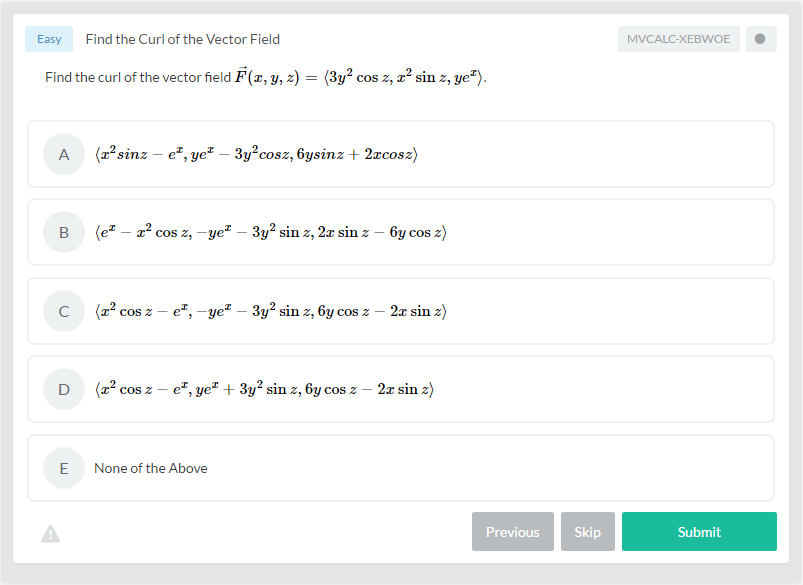
Looking for more Multivariable Calculus practice?
You can find thousands of practice questions on Albert.io. Albert.io lets you customize your learning experience to target practice where you need the most help. We’ll give you challenging practice questions to help you achieve mastery in Multivariable Calculus.
Start practicing here.
Are you a teacher or administrator interested in boosting Multivariable Calculus student outcomes?
Learn more about our school licenses here.


