Introduction to Interpreting Stem Plots
In statistics, descriptive data analysis must always be done first before anything else. This is done so that you can get to know your data, find errors in data collection and data entry, and to find out basic information such as the central tendencies and dispersion characteristics of data. There are many different ways to get to know data, and you are probably most familiar with calculating central tendencies and measures of dispersion.
Another thing we are interested in when describing data is its shape, which can be important for determining whether a variable is appropriate for a particular analysis later on. The stem-and-leaf plot or stem plot, for short, is a way to quickly create a graphical display of quantitative data to get an idea of its shape. Because in AP® Statistics we are interested in normally distributed data, or a bell curve distribution, the stem plot is an easy and fast way to get a general feel of the distribution especially if the data has relatively few observations. Most importantly, the stem plot is useful because it can help with finding the median, mode, and quartiles of data, the range, minimum and maximum values, as well as the most and least frequently occurring observed values in the data.
The stem plot is one method of summarizing univariate data visually. Other ways to summarize univariate data include a histogram and pie chart. The primary advantage of a stem plot is that rather than condensing our data into points or into bars on a graph, we can see the original numerical values of the data. However, as you can probably guess, a main disadvantage of the stem plot is that it is really only useful with relatively small data sets. It would be quite cumbersome to plot out by hand hundreds of values.
Now that we know what stem plots are and how they are useful, how do we actually construct a stem plot? What do we do with a stem plot, or how do we interpret it?
Steps to Interpreting a Stem Plot
First you should know how to construct a stem plot. In a stem plot you have a vertical line dividing the stems from the leaves. The stems are on the left of the vertical line and the leaves are on the right. The stems are usually the first digit of a number. So if you have a value of 25, 2 is the stem that goes on the left of the vertical line and 5 is the leaf that goes on the right.
From the stem plot it should be easy to describe the distribution of the data. You should be able to identify the range, the median, the quartiles, as well as any potential outliers.
Finally, the stem plot should also give you an idea of the shape of the distribution of the data. Is the data normally distributed? Is it shaped like a bell curve?
When interpreting a stem plot you want to find the range, median, quartiles, and interquartile range. Also take note of the general shape of the distribution.
Let’s go through examples of how to create stem plots and how to interpret them.
Example 1
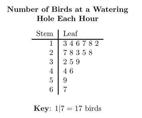
In this example, we have a set of AP® Statistics midterm exam scores.
Since there are relatively few observations, a stem plot would be easy to sketch out and can be useful for describing the general shape of the distribution as well as to find other descriptive statistics.
65, 67, 68, 70, 71, 71, 72, 73, 73, 74, 74, 75, 75, 75, 77, 79, 81, 81, 84, 85, 85, 89, 89, 90, 92
Let’s take the digits in the tens position as the stems and the digits in the ones position as the leaves.
6 | 5 7 8
7 | 0 1 1 2 3 3 4 4 5 5 5 7 9
8 | 1 1 4 5 5 9 9
9 | 0 2
How would you interpret this stem plot?
It appears to show a normal curve, with no real outliers. The midterm exam scores range from 92-65. The median is 75, so 50% of the observations scored below 75 and 50% scored above 75. The mode, the most frequently occurring observation, is 75, like the median.
The quartiles are 71.5 and 84.5, meaning that the middle 50% of the observations fall between these two scores. The interquartile range is 13, meaning that the middle 50% of the exam scores has a range by 13 points, suggesting that they are fairly close together.
From this stem plot we can characterize the distribution as being normally distributed, or a bell curve. That is, there do not seem to be any strange distribution in the data with extreme outliers. Visually, we can make a guess that there are no outliers. However, keep in mind that outliers must be calculated using the 1.5IQR rule.
Example 2
Let’s go through another example of how to interpret stem plots. Here, try to plot the stem plot on your own first.
In this example, we have a stem plot of age-at-first marriage for a sample participating in a focus group.
19, 22, 23, 24, 24, 25, 26, 26, 26, 27, 28, 30, 31, 31, 32, 33, 44
Create a stem and leaf plot using this data, then find the range, median, mode, and interquartile range.
1 | 9
2 | 2 3 4 4 5 6 6 6 7 8
3 | 0 1 1 2 3
4 | 4
From this stem plot it doesn’t appear that there are any outliers, although it is important to recognize that outliers must be determined using the 1.5IQR rule. The distribution appears to be a bell curve. The age at first marriage ranges from 19 years old to 44 years. The median age at first marriage is 26 and the modal category is also 26. The quartiles are Q1 at 24 and Q2 at 31 years old. The IQR is 31-24= 7.
Example 3
In this final example, we have data regarding the number of hours a sample spends on social media on a typical week. It is already set up into a stem plot.
0 | 5 7 9
1 | 0 0 2 9 9 9 9
2 | 1 2 3 4 5 5 6
3 | 0 1 2 3
Are there any outliers? What is the general shape of the data distribution? What is the range and the IQR? What is the mode and median?
From this stem plot, it doesn’t appear as if there are any outliers. The general shape is that of a bell curve. The hours spent on social media ranges from 5 hours to 33 hours. The median is 21 hours and the mode is 19 hours. Quartile 1 is 11 hours and quartile 2 is 25.5 hours. The interquartile range is 25.5 – 11 = 14.5 hours.
Conclusion
Keep in mind that the stem plot is useful for quickly displaying a small set of data visually to observe its general distribution shape, to find the range, the median, the mode, and quartiles including the interquartile range.
Now, while we can gather a lot of information from the stem plot, it is not the final word on determining whether the distribution of our data is actually normally distributed. However, it is a good start when we have a small dataset and we want to quickly sketch the data distribution.
Now that we have walked through three examples of interpreting stem plots, you should be able to easily interpret any stem plots on the AP® exam. The AP® Statistics exam may also ask general questions about stem plots, such as about its uses, its disadvantages and advantages. From this review, you should feel confident not only how to create a stem plot but how to interpret them. Keep in mind that stem plots preserve the original values of numerical variables while showing the shape of the distribution of the data.
Looking for AP® Statistics practice?
Kickstart your AP® Statistics prep with Albert. Start your AP® exam prep today.


