Now that you’ve learned about displacement, velocity, and acceleration, you’re well on your way to being able to describe just about any motion you could observe around you with physics. All that’s left is to learn how these values really play into each other. We know a few ways to move between them, but they’re all pretty limited. What happens if you need to find displacement, but only know acceleration and time? We don’t have a way to combine all of those values yet. Enter the four kinematic equations. 

The Kinematic Equations

The following four kinematic equations come up throughout physics from the earliest high school class to the highest level college course:

Kinematic Equations v=v_{0}+at \Delta x=\dfrac{v+v_{0}}{2} t \Delta x=v_{0}t+\frac{1}{2}at^{2} v^{2}=v_{0}^{2}+2a\Delta x

Don’t let all of these numbers and symbols intimidate you. We’ll talk through each one – what they mean and when we use them. By the end of this post, you’ll be a master of understanding and implementing each of these physics equations. Let’s start with defining what all of those symbols mean. 

The First Kinematic Equation

v=v_{0}+at

This physics equation would be read as “the final velocity is equal to the initial velocity plus acceleration times time”. All it means is that if you have constant acceleration for some amount of time, you can find the final velocity. You’ll use this one whenever you’re looking at changing velocities with a constant acceleration.

The Second Kinematic Equation

\Delta x=\dfrac{v+v_{0}}{2} t

This one is read as “displacement equals final velocity plus initial velocity divided by two times time”. You’ll use this one whenever you don’t have an acceleration to work with but you need to relate a changing velocity to a displacement.

The Third Kinematic Equation

\Delta x=v_{0}t+\frac{1}{2}at^{2}

This one may look a bit scarier as it is longer than the others, but it is read as “displacement equals initial velocity times time plus one half acceleration times time squared”. All it means is that our displacement can be related to our initial velocity and a constant acceleration without having to find the final velocity. You’ll use this one when final velocity is the only value you don’t know yet.

It is worth noting that this kinematic equation has another popular form: x=x_{0}+v_{0}t+\frac{1}{2}at^{2}. While that may seem even more intimidating, it’s actually exactly the same. The only difference here is that we have split up \Delta x into x-x_{0} and then solved to get x on its own. This version can be particularly helpful if you’re looking specifically for a final or initial position rather than just an overall displacement.

The Fourth Kinematic Equation

v^{2}=v_{0}^{2}+2a\Delta x

Our last kinematic equation is read as “final velocity squared equals initial velocity squared plus two times acceleration times displacement”. It’s worth noting that this is the only kinematic equation without time in it. Many starting physicists have been stumped by reaching a problem without a value for time. While staring at an equation sheet riddled with letters and numbers can be overwhelming, remembering you have this one equation without time will come up again and again throughout your physics career.

It may be worth noting that all of these are kinematic equations for constant acceleration. While this may seem like a limitation, we learned before that high school physics courses generally utilize constant acceleration so we don’t need to worry about it changing yet. If you do find yourself in a more advanced course, new physics equations will be introduced at the appropriate times.

How to Approach a Kinematics Problem

So now that we have all of these different kinematic equations, how do we know when to use them? How can we look at a physics word problem and know which of these equations to apply? You must use problem-solving steps. Follow these few steps when trying to solve any complex problems, and you won’t have a problem.

Step 1: Identify What You Know

This one probably seems obvious, but skipping it can be disastrous to any problem-solving endeavor. In physics problems, this just means pulling out values and directions. If you can add the symbol to go with the value (writing t=5\text{ s} instead of just 5\text{ s}, for example), even better. It’ll save time and make future steps even easier.

Step 2: Identify the Goal

In physics, this means figuring out what question you’re actually being asked. Does the question want you to find the displacement? The acceleration? How long did the movement take? Figure out what you’re being asked to do and then write down the symbol of the value you’re solving for with a question mark next to it (t=\text{?}, for example). Again, this feels obvious, but it’s also a vital step.

Step 3: Gather Your Tools

Generally, this means a calculator and an equation. You’ll want to look at all of the symbols you wrote down and pick the physics equation for all of them, including the unknown value. Writing everything down beforehand will make it easier to pull a relevant equation than having to remember what values you need while searching for the right equation. You can use the latter method, but you’re far more likely to make a mistake and feel frustrated that way.

Step 4: Put it all Together

Plug your values into your equation and solve for the unknown value. This will usually be your last step, though you may find yourself having to repeat it a few times for exceptionally complex problems. That probably won’t come up for quite a while, though. After you’ve found your answer, it’s generally a good idea to circle it to make it obvious. That way, whoever is grading you can find it easily and you can easily keep track of which problems you’ve already completed while flipping through your work.

Kinematic Equation 1: Review and Examples

To learn how to solve problems with these new, longer equations, we’ll start with v=v_{0}+at. This kinematic equation shows a relationship between final velocity, initial velocity, constant acceleration, and time. We will explore this equation as it relates to physics word problems. This equation is set up to solve for velocity, but it can be rearranged to solve for any of the values it contains. For this physics equation and the ones following, we will look at one example finding the variable that has already been isolated and one where a new variable needs to be isolated using the steps we just outlined. So, let’s jump into applying this kinematic equation to a real-world problem.

Example 1

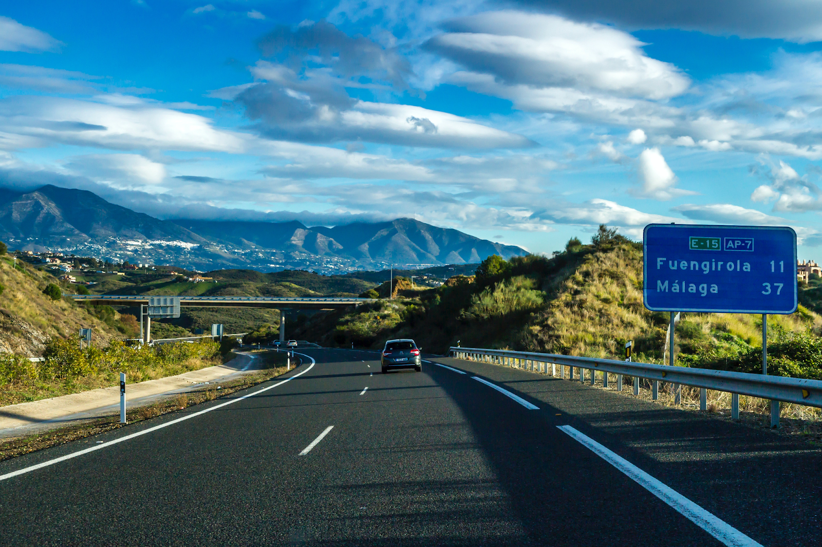
A car sits at rest waiting to merge onto a highway. When they have a chance, they accelerate at 4\text{ m/s}^2 for 7\text{ s}. What is the car’s final velocity?

Step 1: Identify What You Know

We have a clearly stated acceleration and time, but there’s no clearly defined initial velocity here. Instead, we have to take this from context. We know that the car “sits at rest” before it starts moving. This means that our initial velocity in this situation is zero. Other context clues for an object starting at rest is if it is “dropped” or if it “falls”. Our other known values will be even easier to pull as we were actually given numerical values. Now it’s time to put everything into a list.

• v_{0}=0\text{ m/s}
• a=4\text{ m/s}^2
• t=7\text{ s}

Step 2: Identify the Goal

Our goal here was clearly stated: find the final velocity. We’ll still want to list that out so we can see exactly what symbols we have to work with on this problem.

• v=\text{?}

Step 3: Gather Your Tools

We already know which of the kinematic equations we’re using, but if we didn’t, this would be where we search our equation sheet for the right one. Regardless, we’ll want to write that down too.

• v=v_{0}+at

Step 4: Put it All Together

At this point, we’ll plug all of our values into our kinematic equation. If you’re working on paper, there’s no need to repeat anything we’ve put above. That being said, for the purposes of digital organization and so you can see the full problem in one spot, we will be rewriting things here.

• v_{0}=0\text{ m/s}
• a=4\text{ m/s}^2
• t=7\text{ s}
• v=\text{?}

v=v_{0}+at

v=0\text{ m/s}+4\text{ m/s}^2\cdot 7\text{ s}

v=28\text{ m/s}

Example 2

Now let’s get a bit trickier with a problem that will require us to rearrange our kinematic equation.

A ball rolls toward a hill at 3\text{ m/s}. It rolls down the hill for 5\text{ s} and has a final velocity of 18\text{ m/s}. What was the ball’s acceleration as it rolled down the hill?

Step 1: Identify What You Know

Just like before, we’ll make a list of our known values:

• v_{0}=3\text{ m/s}
• t=5\text{ s}
• v=18\text{ m/s}

Step 2: Identify the Goal

Again, our goal was clearly stated, so let’s add it to our list:

• a=\text{?}

Step 3: Gather Your Tools

We already know which equation we’re using, but let’s pretend we didn’t. We know that we need to solve for acceleration, but if you look at our original list of kinematic equations, there isn’t one that’s set up to solve for acceleration:

Kinematic Equations v=v_{0}+at \Delta x=\dfrac{v+v_{0}}{2} t \Delta x=v_{0}t+\frac{1}{2}at^{2} v^{2}=v_{0}^{2}+2a\Delta x

This begs the question, how to find acceleration (or any value) that hasn’t already been solved for? The answer is to rearrange an equation. First, though, we need to pick the right one. We start by getting rid of the second equation in this list as it doesn’t contain acceleration at all. Our options are now:

• v=v_{0}+at
• \Delta x=v_{0}t+\dfrac{1}{2}at^{2}
• v^{2}=v_{0}^{2}+2a\Delta x

Now we’ll need to look at the first list we made of what we know. We know the initial velocity, time, and final velocity. There’s only one equation that has all the values we’re looking for and all of the values we know with none that we don’t. This is the first kinematic equation:

v=v_{0}+at

In this case, we knew the kinematic equation coming in so this process of elimination wasn’t necessary, but that won’t often be the case in the future. You’ll likely have to find the correct equation far more often than you’ll have it handed to you. It’s best to practice finding it now while we only have a few equations to work with.

Step 4: Put it All Together

Like before, we’ll be rewriting all of our relevant information below, but you won’t need to if you’re working on paper.

• v_{0}=3\text{ m/s}
• t=5\text{ s}
• v=18\text{ m/s}
• a=\text{?}

v=v_{0}+at

Although you can plug in values before rearranging the equation, in physics, you’ll usually see the equation be rearranged before values are added. This is mainly done to help keep units where they’re supposed to be and to avoid any mistakes that could come from moving numbers and units rather than just a variable. We’ll be taking the latter approach here. Follow the standard PEMDAS rules for rearranging the equation and then write it with the variable we’ve isolated on the left. While that last part isn’t necessary, it is a helpful organizational practice:

v-v_{0}=at

a=\dfrac{v-v_{0}}{t}

For a review of solving literal equations, visit this post! Now we can plug in those known values and solve:

a=\dfrac{18\text{ m/s}-3\text{ m/s}}{5\text{ s}}

a=3\text{ m/s}^2

Kinematic Equation 2: Review and Examples

Next up in our four kinematics equations is \Delta x=\dfrac{v+v_{0}}{2} t. This one relates an object’s displacement to its average velocity and time. The right-hand side shows the final velocity plus the initial velocity divided by two – the sum of some values divided by the number of values, or the average. Although this equation doesn’t directly show a constant acceleration, it still assumes it. Applying this equation when acceleration isn’t constant can result in some error so best not to apply it if a changing acceleration is mentioned.

Example 1

A car starts out moving at 10\text{ m/s} and accelerates to a velocity of 24\text{ m/s}. What displacement does the car cover during this velocity change if it occurs over 10\text{ s}?

Step 1: Identify What You Know

• v_{0}=10\text{ m/s}
• v=24\text{ m/s}
• t=10\text{ s}

Step 2: Identify the Goal

• \Delta x=\text{?}

Step 3: Gather Your Tools

• \Delta x=\dfrac{v+v_{0}}{2} t

Step 4: Put it All Together

This time around we won’t repeat everything here. Instead, We’ll jump straight into plugging in our values and solving our problem:

\Delta x=\dfrac{v+v_{0}}{2} t

\Delta x=\dfrac{24\text{ m/s}+10\text{ m/s}}{2} \cdot 10\text{ s}

\Delta x=\dfrac{34\text{ m/s}}{2} \cdot 10\text{ s}

\Delta x=17\text{ m/s} \cdot 10\text{ s}

\Delta x=170\text{ m}

Example 2

A ball slows down from 15\text{ m/s} to 3\text{ m/s} over a distance of 36\text{ m}. How long did this take?

Step 1: Identify What You Know

• v_{0}=15\text{ m/s}
• v=3\text{ m/s}
• \Delta x=36\text{ m}

Step 2: Identify the Goal

• t=\text{?}

Step 3: Gather Your Tools

We don’t have a kinematic equation for time specifically, but we learned before that we can rearrange certain equations to solve for different variables. So, we’ll pull the equation that has all of the values we need and isolate the variable we want later:

• \Delta x=\dfrac{v+v_{0}}{2} t

Step 4: Put it All Together

Again, we won’t be rewriting anything, but we will begin by rearranging our equation to solve for time:

\Delta x=\dfrac{v+v_{0}}{2} t

2\Delta x=(v+v_{0})t

t=\dfrac{2\Delta x}{v+v_{0}}

Now we can plug in our known values and solve for time.

t=\dfrac{2\cdot 36\text{ m}}{3\text{ m/s}+15\text{ m/s}}

t=\dfrac{72\text{ m}}{18\text{ m/s}}

t=4\text{ s}

Kinematic Equation 3: Review and Examples

Our next kinematic equation is \Delta x=v_{0}t+\frac{1}{2}at^{2}. This time we are relating our displacement to our initial velocity, time, and acceleration. The only odd thing you may notice is that it doesn’t include our final velocity, only the initial. This equation will come in handy when you don’t have a final velocity that was stated either directly as a number or by a phrase indicating the object came to rest. Just like before, we’ll use this equation first to find a displacement, and then we’ll rearrange it to find a different value.

Example 1

A rocket is cruising through space with a velocity of 50\text{ m/s} and burns some fuel to create a constant acceleration of 10\text{ m/s}^2. How far will it have traveled after 5\text{ s}?

Step 1: Identify What You Know

• v_{0}=50\text{ m/s}
• a=10\text{ m/s}^2
• t=5\text{ s}

Step 2: Identify the Goal

• \Delta x=\text{?}

Step 3: Gather Your Tools

• \Delta x=v_{0}t+\frac{1}{2}at^{2}

Step 4: Put it All Together

\Delta x=v_{0}t+\frac{1}{2}at^2

\Delta x=(50\text{ m/s})(5\text{ s})+\frac{1}{2}(10\text{ m/s}^2)(5\text{ s})^2

\Delta x=250\text{ m}+\frac{1}{2}(10\text{ m/s}^2)(25\text{ s}^2)

\Delta x=250\text{ m}+\frac{1}{2}(250\text{ m})

\Delta x=250\text{ m}+125\text{ m}

\Delta x=375\text{ m}

At this point, it appears that these problems seem to be quite long and take several steps. While that is an inherent part of physics in many ways, it will start to seem simpler as time goes on. This problem presents the perfect example. While it may have been easy to combine lines 4 and 5 mathematically, they were shown separately here to make sure the process was as clear as possible. While you should always show all of the major steps of your problem-solving process, you may find that you are able to combine some of the smaller steps after some time of working with these kinematic equations.

Example 2

Later in its journey, the rocket is moving along at 20\text{ m/s} when it has to fire its thrusters again. This time it covers a distance of 500\text{ m} in 10\text{ s}. What was the rocket’s acceleration during this thruster burn?

Step 1: Identify What You Know

• v_{0}=20\text{ m/s}
• \Delta x=500\text{ m}
• t=10\text{ s}

Step 2: Identify the Goal

• a=\text{?}

Step 3: Gather Your Tools

• \Delta x=v_{0}t+\frac{1}{2}at^{2}

Step 4: Put it All Together

As usual, we’ll begin by rearranging the equation, this time to solve for acceleration.

\Delta x=v_{0}t+\frac{1}{2}at^2

\Delta x-v_{0}t=\frac{1}{2}at^2

2(\Delta x-v_{0}t)=at^2

a=2\dfrac{\Delta x-v_{0}t}{t^2}

Now we can plug in our known values to find the value of our acceleration.

a=2\dfrac{500\text{ m}-20\text{ m/s}\cdot 10\text{ s}}{(10\text{ s})^2}

a=2\dfrac{500\text{ m}-200\text{ m}}{(10\text{ s})^2}

a=2\dfrac{300\text{ m}}{(10\text{ s})^2}

a=2\dfrac{300\text{ m}}{100\text{ s}^2}

a=2\cdot 3\text{ m/s}^2

a=6\text{ m/s}^2

Kinematic Equation 4: Review and Examples

The last of the kinematic equations that we will look at is v^{2}=v_{0}^{2}+2a\Delta x. This one is generally the most complicated looking, but it’s also incredibly important as it is our only kinematic equation that does not involve time. It relates final velocity, initial velocity, acceleration, and displacement without needing a time over which a given motion occurred. For this equation, as with the others, let’s solve it as is and then rearrange it to solve for a different variable.

Example 1

A car exiting the highway begins with a speed of 25\text{ m/s} and travels down a 100\text{ m} long exit ramp with a deceleration (negative acceleration) of 3\text{ m/s}^2. What is the car’s velocity at the end of the exit ramp?

Step 1: Identify What You Know

• v_{0}=25\text{ m/s}
• \Delta x=100\text{ m}
• a=-3\text{ m/s}^2

Note that our acceleration here is a negative value. That is because our problem statement gave us a deceleration instead of an acceleration. Whenever you have a deceleration, you’ll make the value negative to use it as an acceleration in your problem-solving. This also tells us that our final velocity should be less than our initial velocity so we can add that to the list of what we know as well.

• Final velocity will be less than initial.

Being able to know something to help check your answer at the end is what makes this subject a bit easier than mathematics for some students.

Step 2: Identify the Goal

• v=\text{?}

Step 3: Gather Your Tools

• v^{2}=v_{0}^{2}+2a\Delta x

Step 4: Put it All Together

While we generally try to not have any operations going on for the isolated variable, sometimes it’s actually easier that way. Having your isolated variable raised to a power is generally a time to solve before simplifying. This may seem like an arbitrary rule, and in some ways it is, but as you continue through your physics journey you’ll come up with your own practices for making problem-solving easier.

v^{2}=v_{0}^{2}+2a\Delta x

v^{2}=(25\text{ m/s})^{2}+2\cdot (-3\text{ m/s}^{2})\cdot 100\text{ m}

v^{2}=625\text{ m}^{2}/\text{ s}^{2}+2\cdot (-3\text{ m/s}^{2})\cdot 100\text{ m}

v^{2}=625\text{ m}^{2}/\text{ s}^{2}+2\cdot (-300\text{ m}^{2}/\text{ s}^{2})

v^{2}=625\text{ m}^{2}/\text{ s}^{2}-600\text{ m}^{2}/\text{ s}^{2}

v^{2}=25\text{ m}^{2}/\text{ s}^{2}

Now that we have both sides simplified, we’ll take the square root to eliminate the exponent on the left-hand side:

v=5\text{ m/s}

If we remember back at the beginning, we said that our final velocity would have to be less than our initial velocity because the problem statement told us that we were decelerating. Our initial velocity was 25\text{ m/s} which is, indeed, greater than 5\text{ m/s} so our answer checks out.

Example 2

A ghost is sliding a wrench across a table to terrify the mortal onlooker. The wrench starts with a velocity of 2\text{ m/s} and accelerates to a velocity of 5\text{ m/s} over a distance of 7\text{ m}. What acceleration did the ghost move the wrench with?

Step 1: Identify What You Know

• v_{0}=2\text{ m/s}
• v=5\text{ m/s}
• \Delta x=7\text{ m}

We can also make an inference about our acceleration here – that it will be positive. Not every problem will tell you clearly the direction of the acceleration, but if your final velocity is greater than your initial velocity, you can be sure that your acceleration will be positive.

• Positive acceleration

You’ll get better at picking up on subtle hints like this as you continue your physics journey and your brain starts naturally picking up on some patterns. You’ll likely find this skill more and more helpful as it develops and as problems get more difficult.

Step 2: Identify the Goal

• a=\text{?}

Step 3: Gather Your Tools

• v^{2}=v_{0}^{2}+2a\Delta x

Step 4: Put it All Together

We’ll start by rearranging our equation to solve for acceleration.

v^{2}=v_{0}^{2}+2a\Delta x

v^{2}-v_{0}^{2}=2a\Delta x

a\Delta x=\frac{1}{2}(v^{2}-v_{0}^{2})

a=\dfrac{1}{2}\dfrac{v^{2}-v_{0}^{2}}{\Delta x}

As usual, now that we’ve rearranged our equation, we can plug in our values.

a=\dfrac{1}{2}\dfrac{(5\text{ m/s})^{2}-(2\text{ m/s})^{2}}{7\text{ m}}

a=\dfrac{1}{2}\dfrac{25\text{ m}^{2}/\text{s}^{2}-(2\text{ m/s})^{2}}{7\text{ m}}

a=\dfrac{1}{2}\dfrac{25\text{ m}^{2}/\text{s}^{2}-4\text{ m}^{2}/\text{s}^{2}}{7\text{ m}}

a=\dfrac{1}{2}\dfrac{21\text{ m}^{2}/\text{s}^{2}}{7\text{ m}}

a=\frac{1}{2}3\text{ m/s}^{2}

a=1.5\text{ m/s}^2

Again, we can go back to the beginning when we said our acceleration would be a positive number and confirm that it is. 

Problem-Solving Strategies

At this point, you’re likely getting the sense that physics will be a lot of complex problem-solving. If so, your senses are correct. In many ways, physics is the science of explaining nature with mathematical equations. There’s a lot that goes into developing and applying these equations, but at this point in your physics career, you’ll find that the majority of your time will likely be spent on applying equations to word problems. If you feel that your problem-solving skills could still use some honing, check out more examples and strategies from this post by the Physics Classroom or through this video-guided tutorial from Khan Academy.

Conclusion

That was a lot of equations and examples to take in. Eventually, whether you’re figuring out how to find a constant acceleration or how to solve velocity when you don’t have a value for time, you’ll know exactly which of the four kinematic equations to apply and how. Just keep the problem-solving steps we’ve used here in mind, and you’ll be able to get through your physics course without any unsolvable problems.