Introduction

Polynomial functions are a critical topic in AP® Precalculus, forming the foundation for understanding more advanced mathematical concepts. These functions show up everywhere—from predicting the trajectory of a ball to modeling population growth over time.

In this guide, we’ll break down everything you need to know about polynomial functions and their rate of change. You’ll learn about their components, how to find zeros and extrema, and how to analyze their behavior with confidence. We’ll also include a handy quick reference chart to summarize key ideas.

By the end of this article, you’ll have the tools you need to tackle problems from section 1.4 Polynomial Functions and Rates of Change from the AP® Precalculus CED like a pro. Let’s get started!

What Is a Polynomial Function?

Polynomial functions are a key part of AP® Precalculus and appear in many real-world scenarios, like physics and economics. A polynomial function is defined as any equation that can be written in the form:

p(x) = a_nx^n + a_{n-1}x^{n-1} + a_{n-2}x^{n-2} + \dots + a_1x + a_0

Here’s what each part means:

• n: The highest power of x, called the degree of the polynomial.
• a_n: The coefficient of the highest degree term, known as the leading coefficient.
• a_i: Coefficients of the terms, where i ranges from 0 to n. These are real numbers.
• a_0: The constant term, which does not have x.

Example

Let’s take this polynomial:
p(x) = 3x^4 - 2x^3 + 5x^2 - 7x + 9

• The degree is 4 (the highest power of x).
• The leading term is 3x^4, and the leading coefficient is 3.
• The constant term is 9.

Special Case: Constant Polynomial Functions

A constant function, like p(x) = 7, is also a polynomial. Its degree is 0 because it contains no variable x.

Key Characteristics of Polynomial Functions

1. Smooth and Continuous: Polynomial graphs have no sharp corners or breaks.
2. Defined Everywhere: Polynomial functions are valid for all real numbers.

Why Polynomial Functions Matter

Polynomials model countless real-world problems, from predicting population trends to calculating the height of a ball in motion. By mastering them, you’ll build a strong foundation for AP® Precalculus and beyond!

Local and Global Extrema in Polynomial Functions

Polynomial functions often have high and low points on their graphs, known as extrema. These extrema can help us analyze the behavior of a function, which is critical for solving real-world problems or graphing accurately.

Local vs. Global Extrema

• A local maximum is a point where the function’s value is greater than the values of the function at nearby points.
• A local minimum is a point where the function’s value is less than the values of the function at nearby points.
• Among all the local maxima or minima, the greatest local maximum is the global maximum, and the least local minimum is the global minimum.

For example:

p(x) = x^3 - 6x^2 + 9x + 2

• This polynomial has a local maximum and a local minimum.
• If the domain is unrestricted, it has no global maximum or minimum because the cubic function increases or decreases indefinitely.

Even-Degree Polynomial Functions Always Have Global Extrema

Polynomials with even degrees (like x^2 or x^4) always have either a global maximum or a global minimum. Their graphs either open upwards or downwards:

If the leading coefficient is negative, the graph opens downwards, and the function has a global maximum.

If the leading coefficient is positive, the graph opens upwards, and the function has a global minimum.

Zeros and Local Extrema

The zeros of a polynomial function are the points where the graph crosses or touches the x-axis. These zeros play a crucial role in understanding the graph’s behavior, especially when paired with local extrema.

What Are Zeros?

Zeros (or roots) of a polynomial function are the input values x where the function equals zero:
p(x) = 0.

For example, consider:
p(x) = x^3 - 4x^2 + x + 6

To find the zeros, solve:
x^3 - 4x^2 + x + 6 = 0

By factoring or using other techniques, the zeros are found to be x = -1, x = 2, x = 3.

Relationship Between Zeros and Local Extrema

Between every two distinct real zeros of a polynomial function, there must be at least one local maximum or minimum. This is because the graph of the polynomial changes direction as it crosses the x-axis at its zeros.

For example, in the cubic polynomial p(x) = x^3 - 6x^2 + 9x:

• The zeros are x = 0, x = 3.
• A local maximum occurs between these zeros at x = 1.

Visualizing This Concept

Imagine a roller coaster that rises and falls as it travels through hills (local maxima) and valleys (local minima). These hills and valleys must appear between points where the coaster crosses the ground (the zeros).

Points of Inflection and Concavity in Polynomial Functions

Polynomial graphs often change their “shape,” curving upward in some sections and downward in others. These changes in curvature are described using concavity and points of inflection.

What Is Concavity?

Concavity refers to the direction the graph curves:

• A graph is concave up if it looks like a “U” (the slope is increasing).
• A graph is concave down if it looks like an upside-down “U” (the slope is decreasing).

What Are Points of Inflection?

A point of inflection is where the graph changes concavity—from concave up to concave down, or vice versa. These points occur when the rate of change of the function changes from increasing to decreasing or from decreasing to increasing.

Example:

Analyze p(x) = x^3 - 3x^2 + 2x to find the points of inflection and understand the graph’s concavity.

By graphing the function p(x) , we can see where the points of inflection will occur.

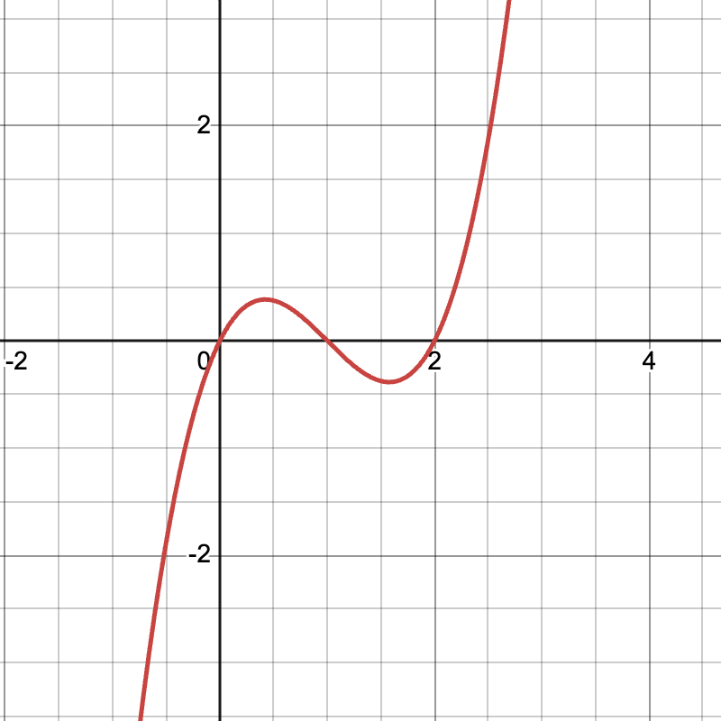
Locate Points of Inflection

• At x = 1, the graph changes from concave up to concave down .
• x = 1 is a point of inflection.

At x = 1, the graph changes concavity, making it a point of inflection.

Conclusion

Polynomial functions are a cornerstone of AP® Precalculus, and mastering them is essential for tackling challenging problems and understanding real-world applications. Here’s what you’ve learned:

• How to break down a polynomial into its key components, like degree, leading term, and zeros.
• The difference between local and global extrema and how to identify them.
• The relationship between zeros and local extrema, as well as the role of points of inflection and concavity.

By combining these concepts, you can analyze and graph any polynomial function with confidence!

Quick Reference Chart for Polynomial Functions

Feature	Definition	How to Identify
Degree	The highest power of x in the polynomial.	Look at the largest exponent.
Leading Term	The term with the highest degree.	Use the term with the largest exponent of x.
Zeros	The points where p(x) = 0.	Factor the polynomial or use the quadratic formula or numerical methods.
Local Extrema	Turning points where the graph changes direction.	Occur between zeros; check intervals where the graph rises or falls.
Global Extrema	The highest (maximum) or lowest (minimum) value of the function over its entire domain.	Only exist for bounded graphs, like those of even-degree polynomials.
Concavity	The direction the graph curves: concave up or concave down.	Test intervals or use graphing tools.
Points of Inflection	Points where the graph changes concavity.	Identify where the graph changes from curving up to curving down, or vice versa.

Keep practicing these concepts by analyzing different polynomial functions. The more you practice, the more intuitive polynomial behavior will become!

With this solid understanding, you’re well on your way to conquering AP® Precalculus and applying these skills to real-world problems. Good luck, and keep exploring math with curiosity!

Need help preparing for your AP® Precalculus exam?

Albert has hundreds of AP® Precalculus practice questions, free response, and an ap precalculus practice test to try out.